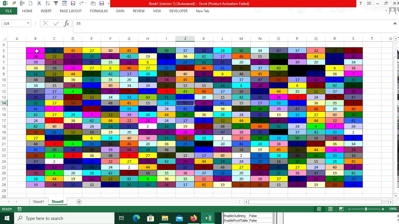
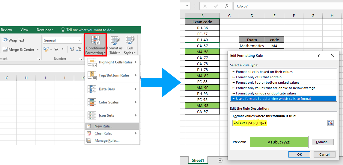
In Excel, you can change the cell color based on the value of another cell using conditional formatting. For example, you can highlight the names of sales reps in column A based on whether their sales are more than 450,000 or not (which is a value we have in cell D2).. In Excel, by using conditional formatting, you can use highlight the entire row. When a condition is true, the row should highlight with the specified color. For example, below, we have a table with the stock data. 1. Highlight a Row Based on a Value (Text) Select the entire table, all the rows and columns. Go to Conditional Formatting > New Rule.

How to count cells based on color 🔴 Count colored cells in excel
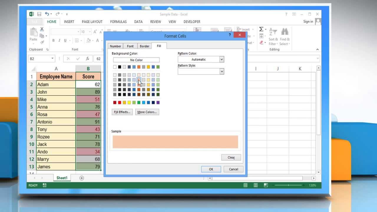
How To Change Background Color In Excel Based On Cell Value Ablebits

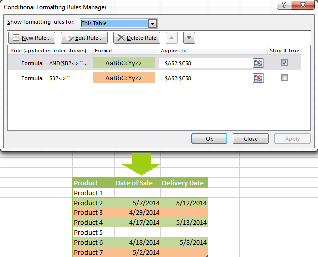
Use the =OR formula to change a row’s color based on several conditions

excel Highlighting the entire row based on cell value Stack Overflow
How to Use Conditional Formatting in Excel to Automatically Change Cell
Vba Tutorial Find The Last Row Column Or Cell In Excel Vrogue
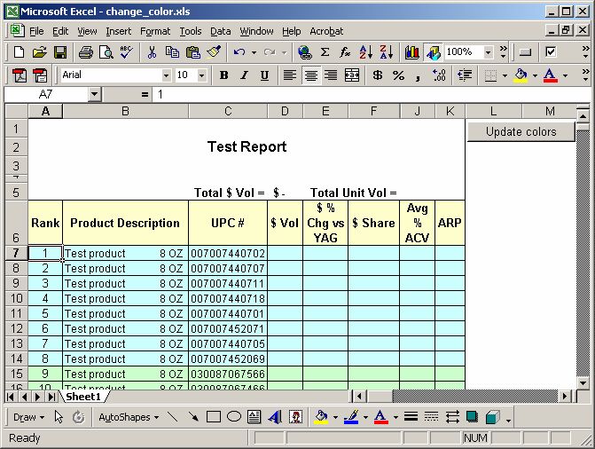
change color of cell in excel based on value Excel background change
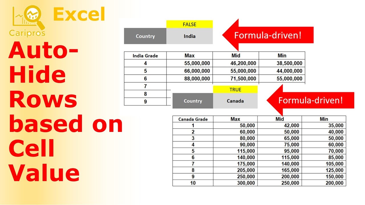
How to Automatically Hide Rows based on Formula driven Cell Value YouTube
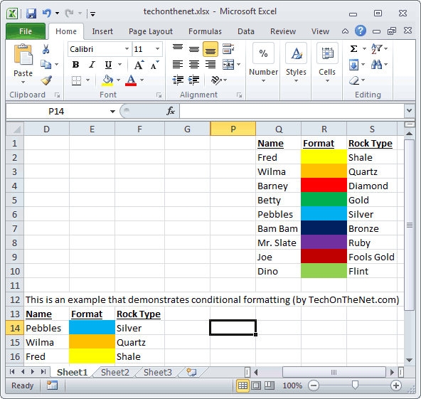
How to Color cell Based on Text Criteria in Excel
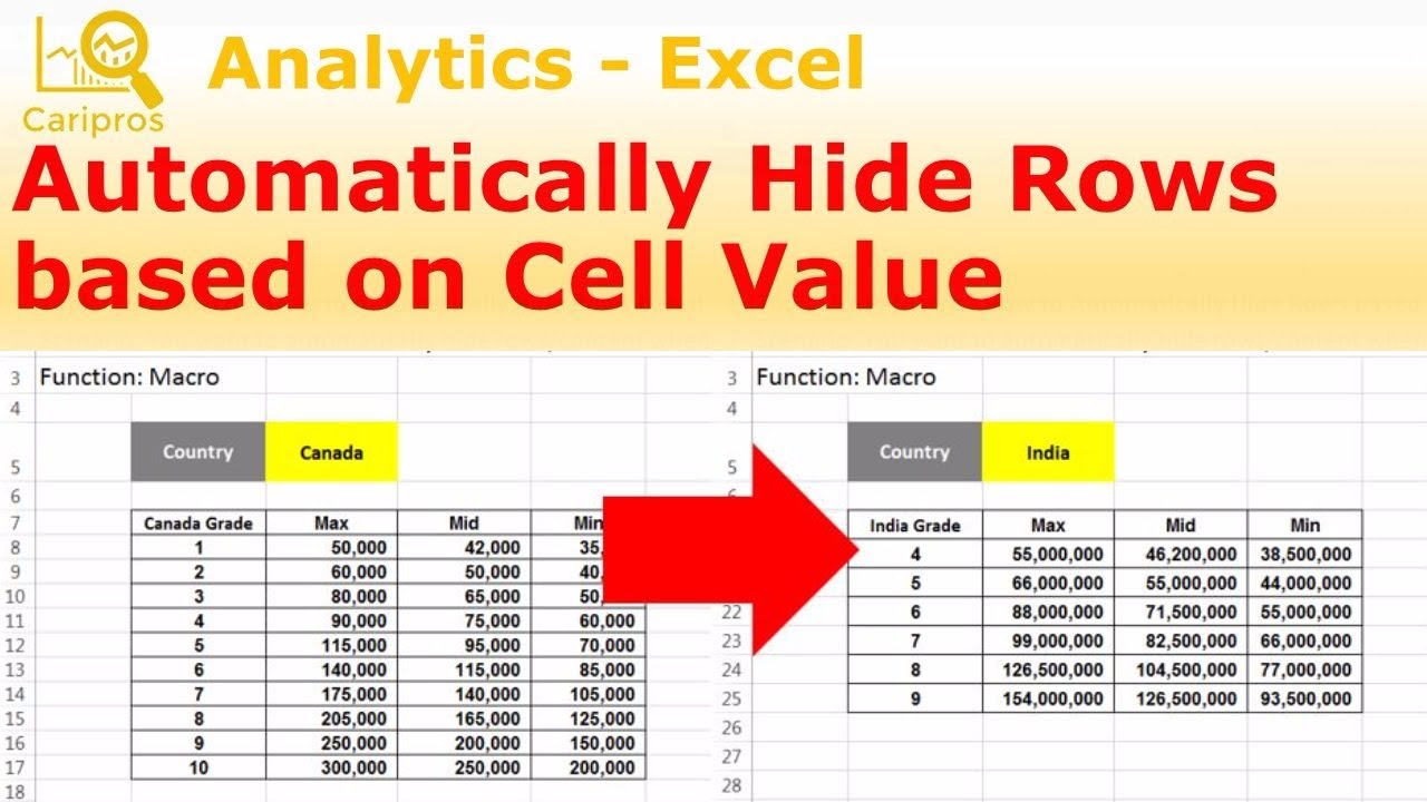
How to Automatically Hide Rows based on Cell Value Macro for Beginner
Can You Color Code In Excel
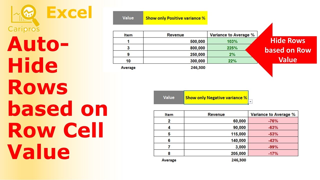
How to Automatically Hide Rows based on Criteria for Row Cell Value
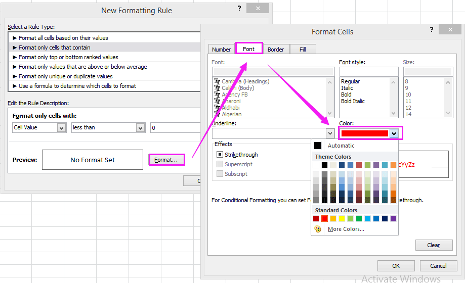
40 Excel Formula Based On Color Image Formulas 21 How To In Cell With A

microsoft excel Row colour change based on text in a cell Super User

2.CONDITIONAL FORMATTING using formulas CORE Concepts Color ROWS
change row color in excel based on cell value Change the row color
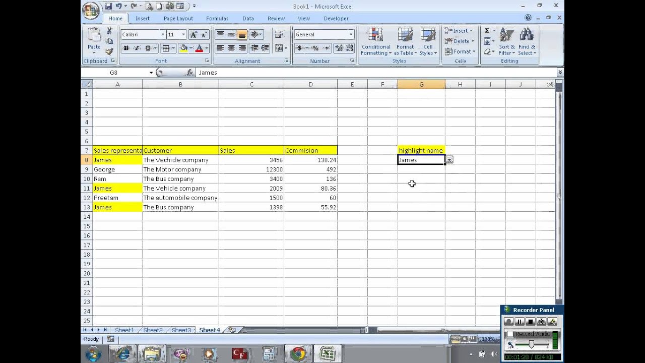
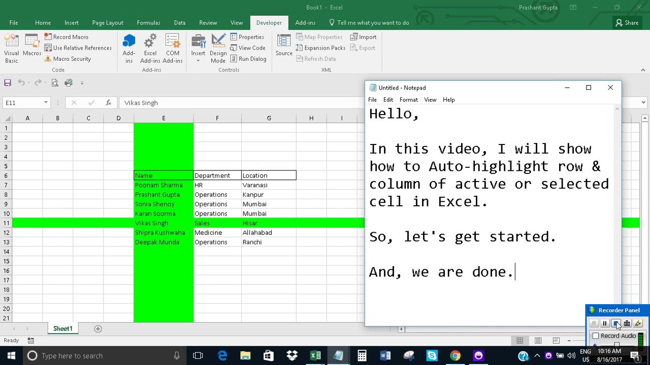
Highlight an entire row in excel based on one cell value YouTube

DatagridView Color row based on cell value Stack Overflow
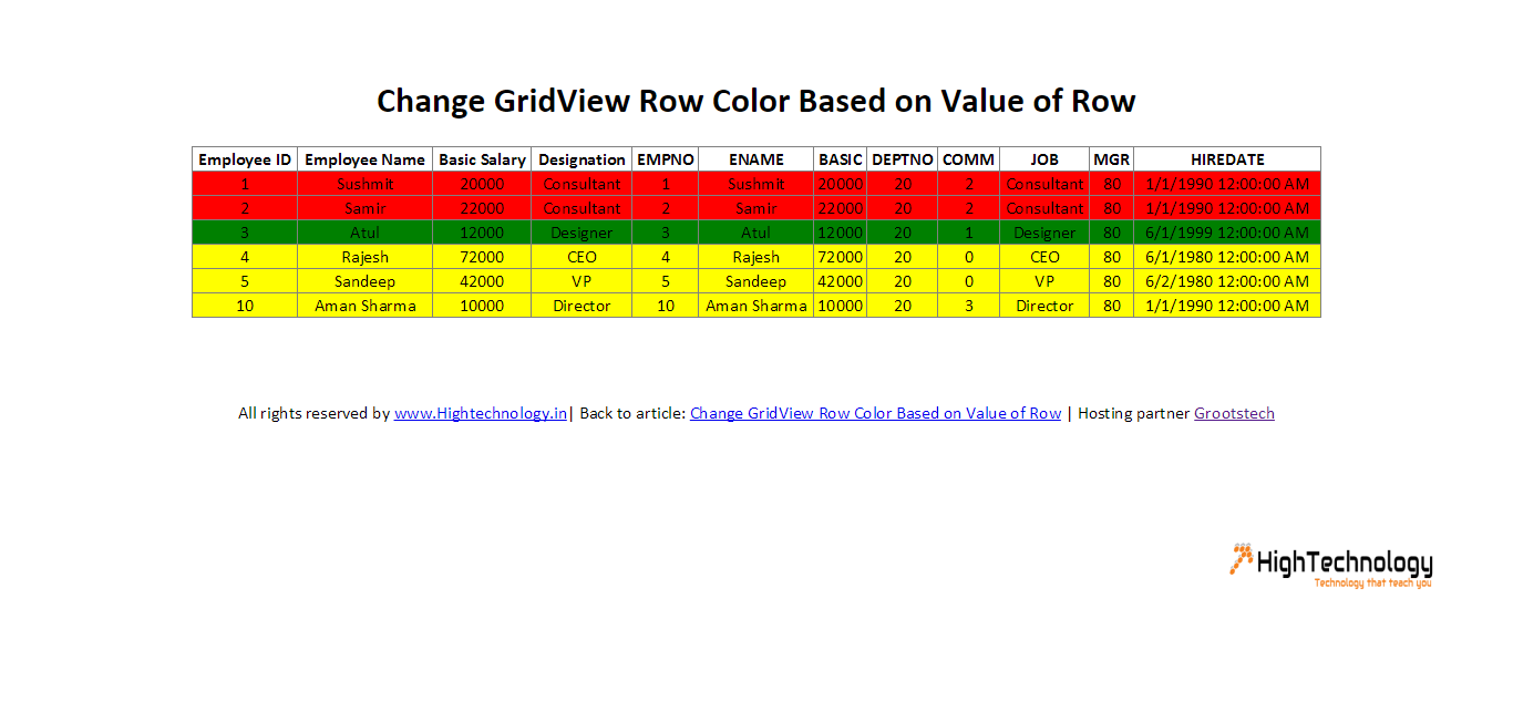
Change GridView Row Color Based on Value of Row

How to Color Alternate Row Based on Cell Value in Excel
In Microsoft Excel, with a few easy steps, you can apply conditional formatting that checks the value in one cell, and applies formatting to other cells, based on that value. For example, if the values in column B greater than 75, make all data cells in the same row blue. This technique can make key information stand out on your Excel worksheets.. Select the cell and hover your mouse cursor in the lower portion of the selected range. A Quick Analysis Toolbar Icon will appear. Click on it. In the Formatting tab, select Greater Than. In the Greater Than tab, select the value above which the cells within the range will change color.
:watermark(assets.rndtech.de/azwaz/watermark-plus.svg,50,50,0)/cloudfront-eu-central-1.images.arcpublishing.com/madsack/DXAH2BLM2UMDVE4CQRDWLXNW2Y.jpg "Downloads VfL Wolfsburg")


